Cerebro: Efficient and Reproducible Model Selection for Deep Learning
This post is about our project Cerebro. Please check the home page at here. You can also find more details in our workshop paper.
Feel like deep learning today? Let’s say you have already purchased one or several beefy machines, set up everything, and found yourself a large enough dataset for the application. It is high time we started training the deep learning model.
The headache of model selection
An immediate problem arises: which neural network architecture should you use? Assume you want convolutional neural networks(CNNs) for your applications. There are AlexNet, VGGNet, InceptionNet, ResNet, Inception-ResNet, MobileNet, SqueezeNet … Say after several hours you finally place your bet, yet you encounter another headache: parameter tuning.
Even with just vanilla stochastic gradient descent(SGD), parameter tuning can still be non-trivial. How do you set the batch size? How large should you set the learning rate? Too large it fails to converge, too small the time cost and your electricity bill become ludicrous. What kind of regularization do you use? If plain L2, how large the regularization should you set? If drop-out, how large should the drop-out proportion be? The list of questions goes on and on.

This huge bottleneck of experimenting model architectures and tuning parameters is called model selection. Unfortunately, there is no axiom for it. It’s very hard, if possible, to determine which configuration gives you the best performance before trying out. Chances are you would need to train a dozen, if not hundreds, of models and benchmark them before reaching the optimal choice.
Alas, favorite deep nets tools like TensorFlow focus on the latency of training one model at a time, not on throughput how many configurations can you try out in unit time. Several parallel execution approaches have been studied. Each has some practical limitations.
The ugliness of un-reproducibility
Reproducibility of the training, which means given the same configuration, the software must yield the same model in the end, is often neglected by web companies. However, it is one of the must-haves of science and a showstopper for many enterprises and domain scientists.
Among various approaches for accelerating deep nets training, some are physically un-reproducible, meaning even if all the pseudo-randomness are saddled, you may still end up with different results.
But don’t worry, Cerebro is here to the rescue.
Review of existing landscapes
In this section, I will briefly introduce two existing forms of parallelism for deep learning training, task, and data parallelism. Feel free to skip the details you are already familiar with this.
-
Task parallelism
-
This is the most straightforward type of parallelism. You use a cluster of machines and dispatch the configurations to them. Every worker has the complete dataset, so there is no communication between the workers during the training.
Pros: Reproducible. Best statistical convergence efficiency. Zero communication overheads while training.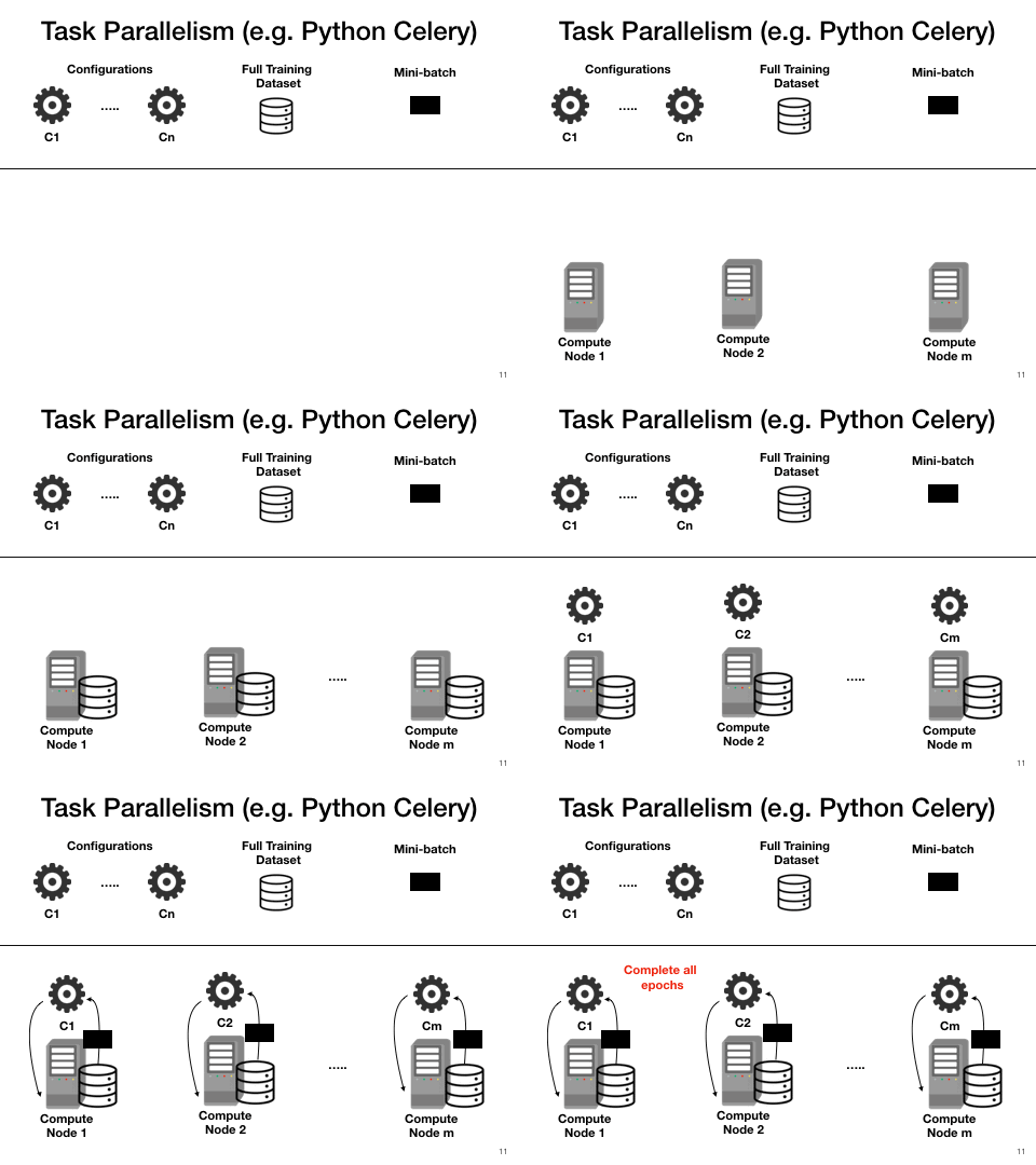
Cons: Storage wastage out of the data replication. Sometimes the dataset can be so big that it no longer fits in single node memory. Down-sampling the dataset will risk over-fitting.
-
This is the most straightforward type of parallelism. You use a cluster of machines and dispatch the configurations to them. Every worker has the complete dataset, so there is no communication between the workers during the training.
-
Data parallelism
- With this type of parallelism, the dataset is partitioned and distributed to the workers. One model configuration is submitted to the cluster at each time. The workers train the model on their partition and update the global weights. I will introduce three methods that reside in this regime: bulk synchronous parallel, parameter server, and decentralized synchronous parallelism. Bulk synchronous parallel(BSP)
-
BSP(AKA model averaging) systems such as Spark and TensorFlow with model averaging parallelize one model at a time. They broadcast the model, train models independently on each worker’s partition, collect all models on the master, average the weights, and repeat this every epoch. Alas, this approach converges poorly; so the application of this method is limited.
Pros: Lowest communication overhead for data parallel training. Good data scalability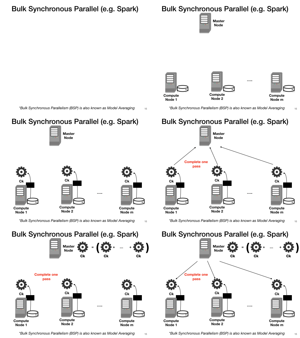
Cons: Poor statistical convergence. -
Parameter server(PS)
-
PS approaches also parallelize one model at a time but at a finer granularity than BSP. Work- ers push gradient updates to the master at each mini-batch and pull the latest model when ready. If the master waits to collect all updates per cycle, it is synchronous; otherwise, if the master continues training whenever it gets an update, it is asynchronous. Asynchronous PS is highly scalable but unreproducible; it often has poorer convergence than syn- chronous PS due to stale updates but synchronous PS has higher overhead for synchronization. All PS-style approaches have high communication costs compared to BSP due to their centralized all-to-one communications at each mini-batch.
Pros: Good data scalability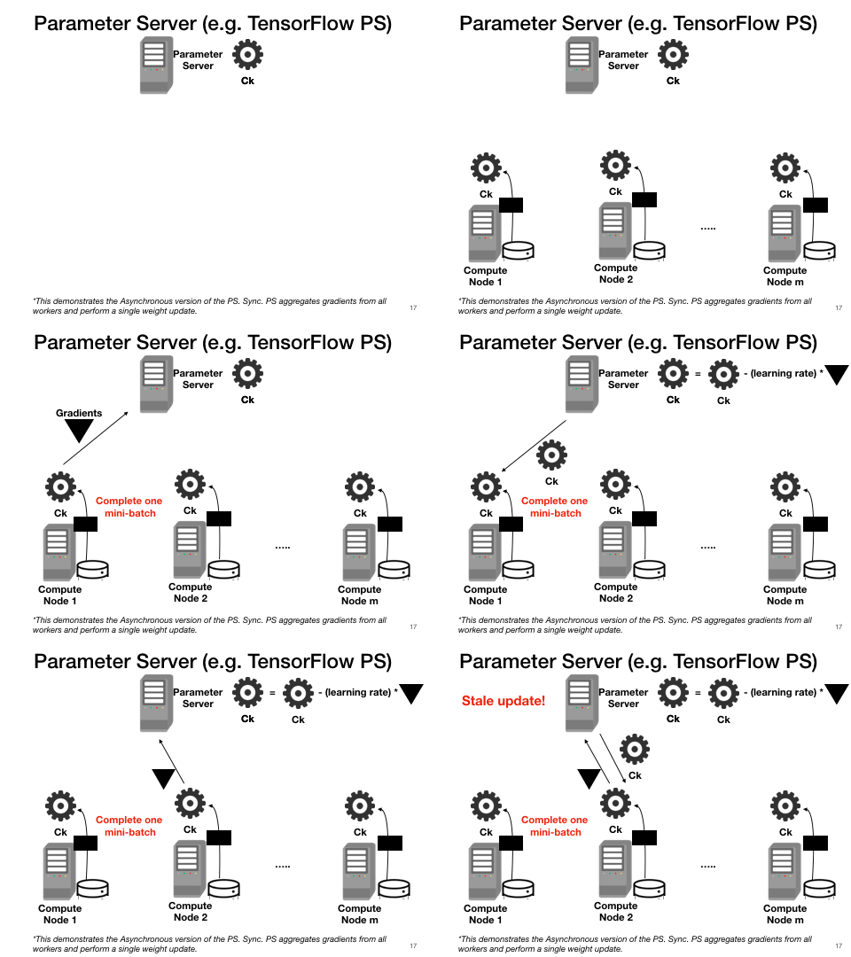
Cons: Poor statistical convergence. Not reproducible(Synchronous-PS alleviates non-reproducibility and stale updates but incurs high overheads due to synchronization). High communication overheads
-
PS approaches also parallelize one model at a time but at a finer granularity than BSP. Work- ers push gradient updates to the master at each mini-batch and pull the latest model when ready. If the master waits to collect all updates per cycle, it is synchronous; otherwise, if the master continues training whenever it gets an update, it is asynchronous. Asynchronous PS is highly scalable but unreproducible; it often has poorer convergence than syn- chronous PS due to stale updates but synchronous PS has higher overhead for synchronization. All PS-style approaches have high communication costs compared to BSP due to their centralized all-to-one communications at each mini-batch.
-
Decentralized synchronous parallelism
-
Decentralized systems such as Horovod adopt HPC-style techniques to enable synchronous all-reduce SGD. It is reproducible and the adopted ring all-reduce algorithm has a time complexity independent of the number of workers for the bandwidth- bound term. However, the synchronization barrier becomes a communication bottleneck.
Pros: Good data scalability. Reproducible.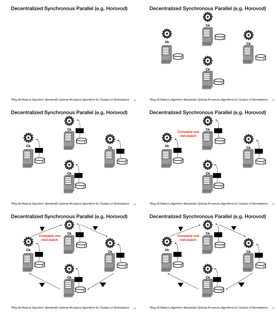
Cons: High communication overheads.
-
Decentralized systems such as Horovod adopt HPC-style techniques to enable synchronous all-reduce SGD. It is reproducible and the adopted ring all-reduce algorithm has a time complexity independent of the number of workers for the bandwidth- bound term. However, the synchronization barrier becomes a communication bottleneck.
Model Hopper Parallelism(MOP): a mixture of task and data parallelism
Cerebro utilizes a combination of task, and data parallelism is the most efficient approach. One key observation is that SGD is robust to data visit order, which means as long as it sees the entire dataset eventually, it does matter in which order the visit may be. Therefore, we purpose Cerebro. The workers now instead of exchanging weights, sending the checkpointed models to each other after each epoch of training. This requires minimal disk storage and trivial communication.
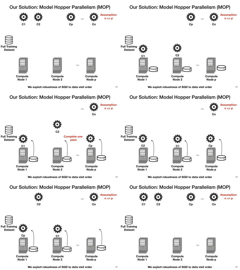
With such design, Cerebro should be highly data-scalable, reproducible , efficient and have perfect convergence speed. We also envision Cerebro to be the narrow waist between the AutoML procedures and the various deep learning frameworks such as TensorFlow, PyTorch. (A) and (B) of the following figure demonstrate the power of Cerebro and (C) shows its position in the entire tool-chain of deep learning.

Experiments on ImageNet
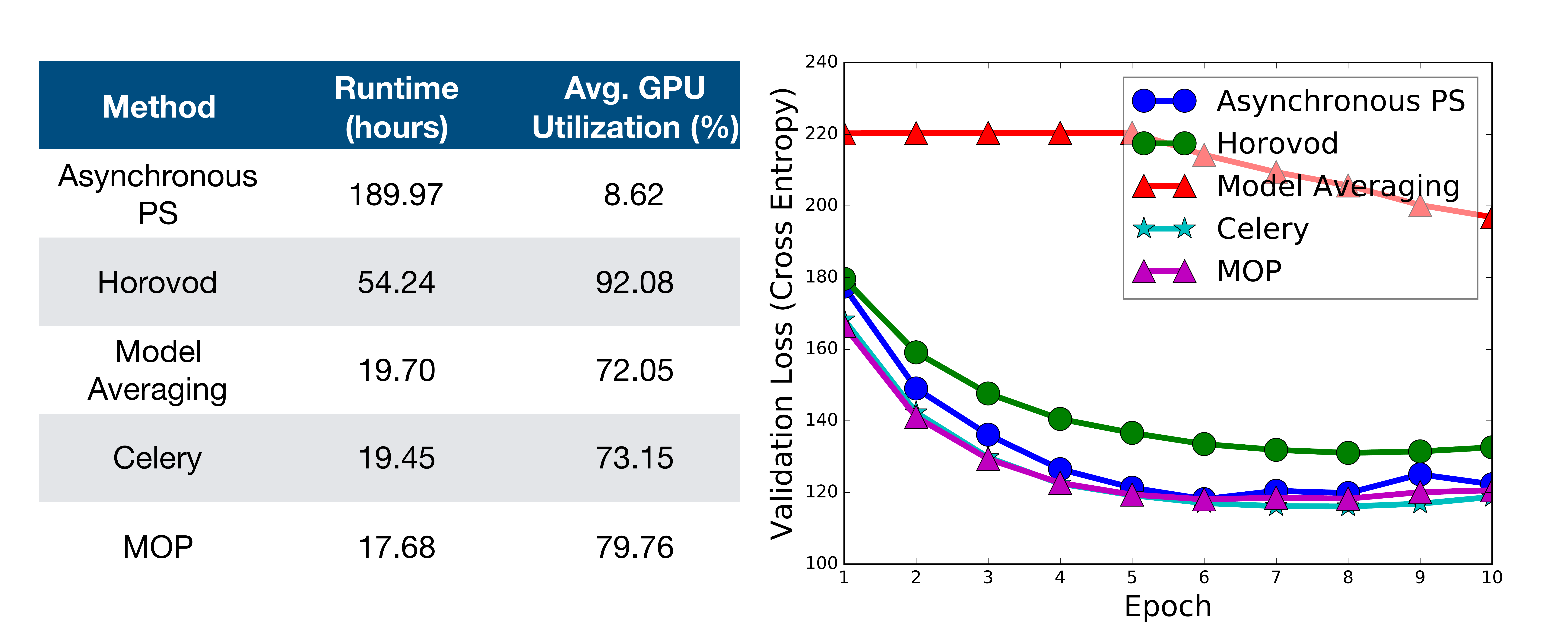
Now it is time to show you some experiment results. We compare a prototype implementation of MOP on TensorFlow to many state-of-the-art systems on an 8-node GPU cluster with Nvidia P100 GPUs. We train 16 models on ImageNet for 10 epochs: 2 architectures (VGG16 and ResNet50), 2 batch sizes (32 and 256); 2 learning rates (10E−4 and 10E−6 ), and 2 regularizers (10E-4 and 10E-6).
The following figure shows the makespans, average GPU utilization, and learning curves of the best model from each system.
Takeaways
- MOP is over 10x faster than TF’s in-built asynchronous PS.
- MOP is also 3x faster than Horovod. The high GPU utilization is because Horovod’s communication utilizes GPU kernels.
- MOP’s runtime is comparable to TF’s model averaging and task parallelism.
- Model averaging converges very slowly.
- Celery and MOP have the best learning curves but note that Celery has 8x the memory/storage footprint as MOP due to dataset copies.
- Overall, MOP is the most resource-efficient and still offers accuracy similar to sequential SGD.
The system is open-sourced and available at Cerebro. Hopefully, Cerebro can one day help you, my friend, the master of the black arts of deep learning. Have a nice day!